Shaped Transformer
Understanding Transformer
How can one learn Transformer?
The Transformer Architecture (introduced in the paper Attention is All You Need) is one of the most successful models in deep learning and the backbone of what made the “ChatGPT moment” possible. Because of its importance and impact, there are already many high-quality explanations of what the model is, how it works, and even annotated code implementation of it. These days, most developers don’t need to implement Transformers from scratch because libraries like HuggingFace Transformers provide easy-to-use classes and methods. Yes, there are plenty of things to build on top of the architecture! Still, I think it is worth having a great understanding of Transformer Model, beyond intuitive, abstract level. In fact one of the best way to learn Transformer, as Feynman said, is to build one yourself from scratch to really understand and appreciate all the underlying techniques and modules that form the base of the ChatGPT era.
How is this different from other content?
Before I start, I do strongly recommend reading other resources as well. However note that each sources has different layers of abstraction (or depth of explanation). The paper itself is fairly straightforward but not chronologically ordered, so it can be hard to follow in details.
The Illustrated Transformer is beginner-friendly, abstracting away many implementation details and excels at explaining the overall big picture. On the other hand, The Annotated Transformer is very deep, building the entire architecture end to end in PyTorch. But since it follows the paper’s order (which isn’t chronological) and leaves out some explanations, readers who only have an abstract understanding of the model may feel overwhelmed or questionable.
Also note that Transformer is not a single monolithic block—it’s made up of many modularized layers (tokenization, positional encoding, encoder-decoder model, self-attention, cross-attention, etc.). Unless you already have a solid background in deep learning and NLP, it’s hard to fully understand all the pieces in one go. You’ll often need additional resources, and repeated exposure, to get comfortable with it.
While there are many great explanations of the mathematics and abstract concepts, I think the end-to-end shape changes and detailed explanation of code implementation are often missing. This blog post specifically aims to enhance the reader’s intuition about what the input actually looks like in real code, how it gets transformed step by step, and how it eventually can successfully predict the “next token”.
Hopefully this helps you form a more concrete understanding of the architecture and makes the code easier to read and implement :)
Commonly Used Parameters
Before we talk about shape transformation, it is helpful to understand the names of the parameter/notations. It will help the code readability. If you are familiar with the paper and the parameters used, feel free to skip this section.
$N$ , $b$, or nbatches
The Paper use the expression $N$ but in code, it is expressed as nbatches.
The reason why you may be confused about nbatches in code implementation from Annotated Transformer is because most explanation (including the original paper) omit about it.
The most representative image of Transformer is usually
- One head from one batch or
- Multi-Head from one batch
but they don’t explicitly tell there arenbatchesbatches processed parallel for each batch.
The reality is, $N$ sentences are put into batch and passed as input. But this doesn’t change or introduce anything new to the original architecture we know. Still it’s worth noting that nbatches mean the number of sentences being processed per batch. It will appear in the code several times.
Ex. let’s say $N=3$. That means we have $3$ sentences per batch.
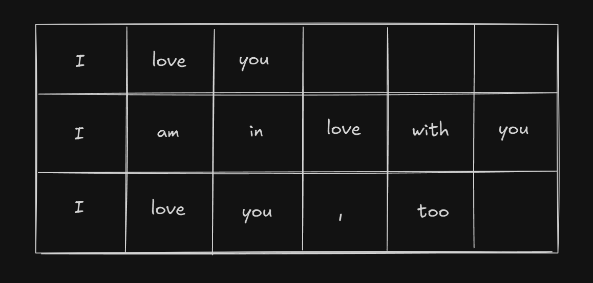
$S$ or n_seq
n_seq means the number of tokens in one sentence. Since Transformer utilizes parallel processing, we need to pre-define (statically) the length of the sentence. Usually we define it based on the longest sentence.
For example,
I love you            --3
I am in love with you --6
I love you, too       --5
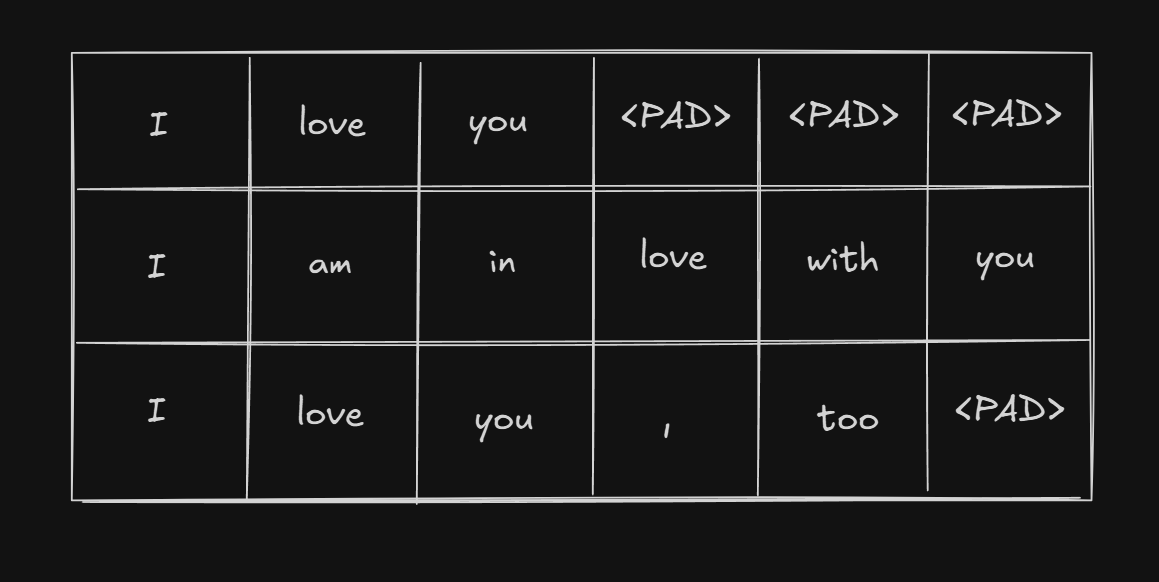
in this case, since the longest sentence in the batch is $6$, we can set n_seq = 6.
For the sentences that have less tokens than 6 will be filled with mask. We will see how mask(padding) is implemented later in this post.
$d_{\text{model}}$ or d_model
d_model is the dimensionality of the residual stream, i.e., the vector size that represents each token throughout the Transformer.
All major components, including Embedding, Attention, and Feed-Forward layers, produce outputs of shape (N, S, d_model). This uniform dimension ensures that residual connections (x = x + sublayer(x)) can be applied seamlessly across all sublayers.
In the original paper, d_model was set to 512.
$vocab$ or vocab
vocab is number of all token (or token ID). It depends on how you tokenize it.
(I think prior resources didn’t explain about the exact input of Transformer architecture clearly but I think it’s worth noting.)
First, even before the transformer process begins, there something called a Tokenizer which is independent from the Transformer Architecture. The tokenizer splits raw sentences into seqeunce of tokens.
For example if the raw sentence input was I love you, Tokenizer would divide it into tokens,
["I", "love", "you"]
and using the $vocab$ dictionary, we map the tokens with its correspoining token id (one-on-one match)
[0, 1, 2]
Now this (sequences of token id) is the input of the Transformer Architecture.
Then you might ask what the input of Transformer is.
The very first step of Transformer is Embedding and this is done by selecting the row from W_emb using the token ID as a key: W_emb[token ID]
token_id = 1 ("love")
→ W_emb[1] = [0.13, -0.25, 0.91, ..., 0.07]
Since the vector representation of token has size of $d_\text{model}$ (as mentioned above) The shape of $W_\text{emb}$ will be $(vocab, d_{\text{model}})$.
tldr:
vocabmeans number of all possible tokens, which depends on the Tokenizer.- After the token is converted into token id, the sequence of token ids become the actual “input” of the Transformer Architecture (The most left, below from the Transformer Architecture image)
Parameters specifically used During Attention Calculation
Below are the parameters only seen in Attention Calculation (Self-Attention and Cross-Attention)
$H$, $h$, or h
h is a hyperparameter which means the number of head of Multi-Head Attention.
In the original paper, researchers set it as h = 8.
$d_k$ or d_k
d_k is the vector size of key($K$) representation of each token.
We will look into more detail about how shape transforms during Multi-Head Attention in the upcoming section, but to shortly address, $Q$(query) and $K$(key) are matrix multiplied($QK^T$) to get the Attention Score. Therefore d_q must be the same as d_k.
In the original paper, d_k is set to d_model // h($512/8 = 64$). While d_k does not strictly have to equal d_model // h, this configuration ensures that the concatenated output of all attention heads matches the original d_model dimension. This structural alignment allows the output to be added directly to the residual connection without additional linear projections or dimension adjustments, thereby maximizing computational efficiency.
$d_v$ or d_v
d_v is the dimension of the value($V$) vector for each token.
After the attention weights are calculated, they are multiplied by the Value matrix $V$. This process yields a new set of vectors, each with dimension d_v, that now holds the contextual information from the sequence. This output is then used to help predict the next token.
(Don’t worry if this sounds too compact. I will explain it in more detail later.)
In the original “Attention Is All You Need” paper, the authors set d_v = d_k = d_q. However, while d_k must equal d_q, it’s not required for d_v to be the same size. This is simply another design choice. I will also explain later in this post when d_v != d_k is acceptable.
How Shape Changes, End to End (w/ Code Example)
When we encounter the code implementation of Transformer Architecture, all kinds of view(), transpose(), reshape() methods are frequently used, hindering what are being changed , what it implies, and why we need to do it. After all, if you understand there is a general order within the parameters and the shape form all has its meanings, code readability can significantly enhance.
Before we start, a simple but effective tip is to remember that most calculations
(token embedding, self-attention, feed-forward, etc.) in Transformer are applied per token(d_model).
In practice, the input shape is (nbatches, n_seq, d_model), which means each sequence has n_seq tokens and each batch has nbatches sentences. Almost all operations are performed independently on each of these tokens (in parallel). So you can think of it as running the same function nbatches × n_seq times in parallel.
Now, let’s explore the journey from the very first embedding to the last output (next token) and see how the shape changes and what they all mean. (In most paper or images, they often omit nbatches or h for clarity but I will explain including all the parameters). Then we will see how code is actually written to match these shapes. We won’t cover all code, just the shape transformation parts, for simplicity. Also, to give you a clear intuition of how everything is working, I will use the three following sentences I used above. Code can be found in … :
0. Input (both Encoder & Decoder)
As mentioned above, this is a step before the transformer architecture even starts. It’s a process to convert raw sentences into sequence of tokens. For example, based on GPT-4o & GPT-4o mini tokenizer provided by OpenAI,
I love you
I am in love with you
I love you, too
(we will use these three sentences in each step until the end of the architecture)
are converted into discrete tokens:
In code, we use tokenizer.tokenizer module:
def tokenize(text, tokenizer):
    return [tok.text for tok in tokenizer.tokenizer(text)]
We use padding tokens(PAD) to keep the length of all n_seq same (which is crucial for matrix calculation). If we set n_seq to 6, the padding will fill as below:
These tokens converted to token ids will be
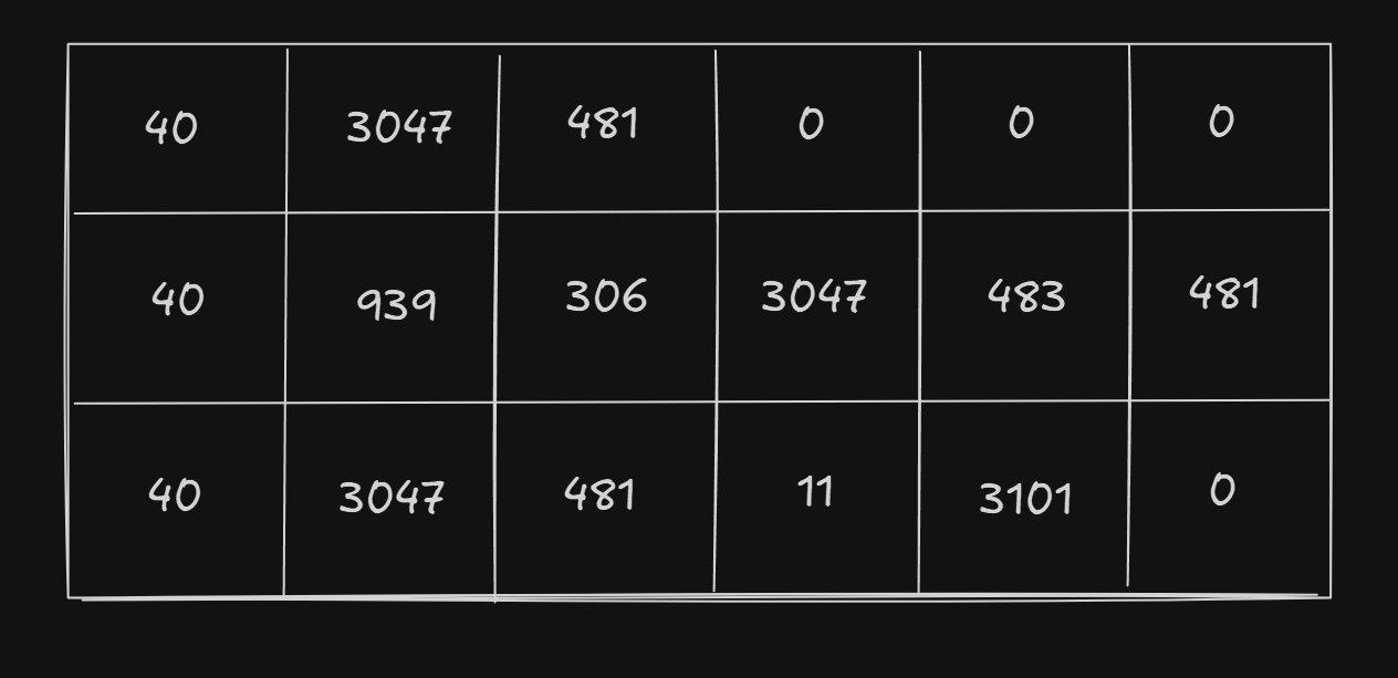
(according to GPT-4o tokenizer)
This will be our exact starting point (input) for Transformer Architecture.
Let’s see how this is implemented as code:
class Batch:
    """Object for holding a batch of data with mask during training."""
    def __init__(self, src, tgt=None, pad=2):  # 2 = <blank>
        self.src = src
        self.src_mask = (src != pad).unsqueeze(-2)
        if tgt is not None:
            self.tgt = tgt[:, :-1]
            self.tgt_y = tgt[:, 1:]
            self.tgt_mask = self.make_std_mask(self.tgt, pad)
            self.ntokens = (self.tgt_y != pad).data.sum()

    @staticmethod
    def make_std_mask(tgt, pad):
        "Create a mask to hide padding and future words."
        tgt_mask = (tgt != pad).unsqueeze(-2)
        tgt_mask = tgt_mask & subsequent_mask(tgt.size(-1)).type_as(
            tgt_mask.data
        )
        return tgt_mask
In this code, padding token(<blank>) is set to ‘2’.
This is just because the authors of Annotated Transformer set <blank> as the third special token (specials=["<s>", "</s>", "<blank>", "<unk>"])
shape: (nbatches, n_seq)
1. Encoder Embedding Layer
1-1. Token Embedding
Now the Transformer Architecture starts.
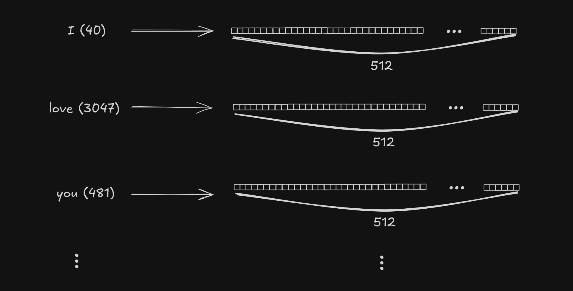
First thing we do is we embed all token in sequences within a batch.
Embedding matrix W_emb shape is (vocab, d_model). In the original paper d_model is set to 512.
Input((nbatches, n_seq)) will use W_emb as a lookup table and replace the token id into d_model dimension, which makes the scalar token id into d_model dimension vector for each token.
After embedding, we scale the elements in d_model by multiplying it with $\sqrt{d_\text{model}} = \sqrt{512}$. Original paper doesn’t explain the reason clearly but based on this, it seems they are multiplying to keep/strengthen the token embedding information even after Positional Embedding is added. Since it’s just scalar multiplication, this procedure doesn’t change the shape.
shape: (nbatches, n_seq_src) → (nbatches, n_seq_src, d_model)
Back to our example, the sentence “I love you”(40 ,3047, 481, 0, 0, 0) will extract W_emb[40], W_emb[3047], W_emb[481], and W_emb[0].
| token | token id | d_model = 512 |
|---|---|---|
[PAD] | 0 | [ 0.00, 0.00, 0.00, 0.00, 0.00, 0.00, 0.00, 0.00, ... ] |
I | 40 | [ 0.12, -0.07, 0.91, -0.04, 0.26, 0.03, -0.18, 0.55, ... ] |
love | 3047 | [ 0.33, 0.25, -0.48, 0.18, -0.09, 0.41, 0.07, -0.22, ... ] |
you | 481 | [-0.55, 0.19, 0.07, 0.92, -0.14, 0.08, 0.36, -0.02, ... ] |
am | 939 | [ 0.41, 0.05, 0.36, -0.33, 0.22, -0.17, 0.10, 0.04, ... ] |
in | 306 | [ 0.29, -0.15, -0.04, 0.22, -0.11, 0.09, -0.27, 0.30, ... ] |
with | 483 | [-0.21, 0.56, 0.02, 0.44, 0.05, -0.08, 0.12, -0.19, ... ] |
, | 11 | [ 0.77, -0.10, -0.13, -0.26, 0.15, 0.06, -0.05, 0.02, ... ] |
too | 3101 | [ 0.04, 0.88, -0.29, 0.13, -0.06, 0.21, -0.12, 0.44, ... ] |
After replacing based on the W_emb lookup table, “I love you” would be
E[0, 0, :] = [ 0.12, -0.07,  0.91, -0.04,  0.26,  0.03, -0.18,  0.55, ... ]   # "I"    (id=40)
E[0, 1, :] = [ 0.33,  0.25, -0.48,  0.18, -0.09,  0.41,  0.07, -0.22, ... ]   # "love" (id=3047)
E[0, 2, :] = [-0.55,  0.19,  0.07,  0.92, -0.14,  0.08,  0.36, -0.02, ... ]   # "you"  (id=481)
E[0, 3, :] = [ 0.00,  0.00,  0.00,  0.00,  0.00,  0.00,  0.00,  0.00, ... ]   # [PAD]  (id=0)
E[0, 4, :] = [ 0.00,  0.00,  0.00,  0.00,  0.00,  0.00,  0.00,  0.00, ... ]   # [PAD]  (id=0)
E[0, 5, :] = [ 0.00,  0.00,  0.00,  0.00,  0.00,  0.00,  0.00,  0.00, ... ]   # [PAD]  (id=0)
Of course other two sentences in the batch, “I am in love with you” and “I love you, too” also will go through the same process.
1-2. Positional Embedding
We won’t go into detail about positional embedding in this post, since itself is a post-worth concept. I recommend this post for better understanding of Positional Embedding. Since our main focus here is to see how the shapes change, I will explain mainly on that point of view.
To briefly explain, Positional Embedding is adding same(d_model)-sized vector to each embedded token to preserve the positional information. Unlike other sequence neural networks such as LSTM or RNN, Transformer calculates all tokens parallel. Therefore, if it doesn’t have positional information added, it wouldn’t know the order of the token. While using $\sin$ and $\cos$ functions are not the only way to preserve positional information, it is known to be a helpful way to do that.
We add the positional information of d_model to each embedded tokens and since they have the same shape, the shape does not change.
shape: (nbatches, n_seq_src, d_model) → (nbatches, n_seq_src, d_model)
Back to our example, “I love you” has three positions.
PE[0, :] = [ 0.00,  1.00,  0.00,  1.00,  0.00,  1.00,  0.00,  1.00, ... ]   # pos=0
PE[1, :] = [ 0.84,  0.54,  0.84,  0.54,  0.84,  0.54,  0.84,  0.54, ... ]   # pos=1
PE[2, :] = [ 0.91, -0.42,  0.91, -0.42,  0.91, -0.42,  0.91, -0.42, ... ]   # pos=2
PE[3, :] = [ 0.14, -0.99, 0.14, -0.99, 0.14, -0.99, 0.14, -0.99, ... ] # pos=3
PE[4, :] = [-0.76, -0.65, -0.76, -0.65, -0.76, -0.65, -0.76, -0.65, ... ] # pos=4
PE[5, :] = [-0.96, 0.28, -0.96, 0.28, -0.96, 0.28, -0.96, 0.28, ... ] # pos=5
We add the PE with E for every token:
E+PE[0, 0, :] = [ 0.12+0.00, -0.07+1.00,  0.91+0.00, -0.04+1.00, ... ]   # "I"
           = [ 0.12, 0.93, 0.91, 0.96, 0.26, 1.03, -0.18, 1.55, ... ]

E+PE[0, 1, :] = [ 0.33+0.84, 0.25+0.54, -0.48+0.84, 0.18+0.54, ... ]     # "love"
           = [ 1.17, 0.79, 0.36, 0.72, 0.75, 0.95, 0.91, 0.32, ... ]

E+PE[0, 2, :] = [-0.55+0.91, 0.19-0.42, 0.07+0.91, 0.92-0.42, ... ]     # "you"
           = [ 0.36, -0.23, 0.98, 0.50, 0.77, -0.34, 1.27, -0.44, ... ]

E+PE[0, 3, :] = [ 0.00+0.14, 0.00-0.99, 0.00+0.14, 0.00-0.99, ... ]     # [PAD] at pos=3
           = [ 0.14, -0.99, 0.14, -0.99, 0.14, -0.99, 0.14, -0.99, ... ]

E+PE[0, 4, :] = [ 0.00-0.76, 0.00-0.65, 0.00-0.76, 0.00-0.65, ... ]     # [PAD] at pos=4
           = [-0.76, -0.65, -0.76, -0.65, -0.76, -0.65, -0.76, -0.65, ... ]

E+PE[0, 5, :] = [ 0.00-0.96, 0.00+0.28, 0.00-0.96, 0.00+0.28, ... ]     # [PAD] at pos=5
We can see that even though the padding tokens have no semantic meaning, they still receive a unique positional signal before being processed by the Transformer layers.
As always, remember this process is done by all sequences in the batch! (which means this process is parallelly done in the sentences “I am in love with you” and “I love you, too” as well!)
Since attention itself doesn’t have the ability to consider positions, we add additional information to each tokens. Since the positional embedding vector is also d_model size vector, we simply add them and there is no shape change.
2. Encoder Layer
Now we move to the Encoder Layer. Code implementation of Encoder (and Decoder) Layer in code seems like a matryoshka doll (module inside a module inside a module…) but I will try to explain the big picture as clearly as possible.
In the blueprint, Encoder is consisted of $N$ Layers of Encoder Layer. (Note that Encoder and Encoder Layer are NOT the same! Also note that $N$ here and nbatches are totally different, independent concepts!) In the original paper $N=6$ which means we go over the Encoder layer 6 times in a single process.
Each Encoder Layer has two Sublayers: Self-Attention Sublayer first and then Feed Forward Network($FFN$) Sublayer. After each sublayers are passed, they are connected to a residual stream and then layer-wise normalized(LayerNorm).
In code, Sublayers are the most fundamental building blocks in Encoder-Decoder structure of Transformer Architecture. The two types of sublayers are already mentioned above.
Now that we went over the modules inside Encoder in a brief top-down approach, we will first go over the shape/dimension changes in Self-Attention Sublayer, then Feed Forward Network Sublayer and will expand further.
2-1. Multi-Head Self Attention (MHA)
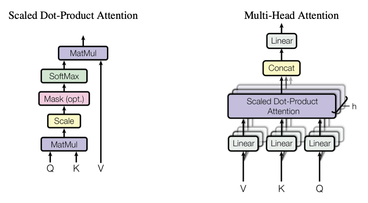
When the input enters an Encoder Layer, its first destination is the Self-Attention sublayer.
To understand what happens here, we need to talk about Multi-Head Attention.
Though this post isn’t a deep theoretical dive, the core idea is simple: Instead of calculating attention just once, we use multiple “attention heads.” Think of it like having several experts look at the same sentence; each expert (or head) can focus on different relationships between words. Each head has its own set of learned weights (W_Q, W_K, W_V) to find these different relationships. In the original paper, they use 8 heads (h=8).
Mathematically we represent Attention calculation as
$$\text{Attention}(Q, K, V) = \text{softmax}\left( \frac{QK^T}{\sqrt{d_k}} \right) V$$
This module is one of the most complicated part in Transformer so we will look in detail, step by step. The goal is to get a clear sense of how shape changes during each process. We are going to divide the Self-Attention process into 8 minor steps.
We start from input from 1-2
shape: (nbatches, n_seq_src, d_model) (shapes unchanged)
x2-1-1. Project to Q,K,V
In Self Attention, inputs are copied and passed to three different Projections which each has independent weights($W_Q, W_K, W_V$).
Mathematically put:
$$
\begin{aligned}
q_i &= h_i \cdot W_Q \
k_i &= h_i \cdot W_K \
v_i &= h_i \cdot W_V
\end{aligned}
$$
The size of the weights (without considering the heads) are all (d_model, d_model). This happens “per token” and the vector size of the token stays the same so shape does not change.
shape: (nbatches, n_seq_src, d_model) (shapes unchanged)
For example, the sentence “I love you” (with 3 <PAD> tokens) will be: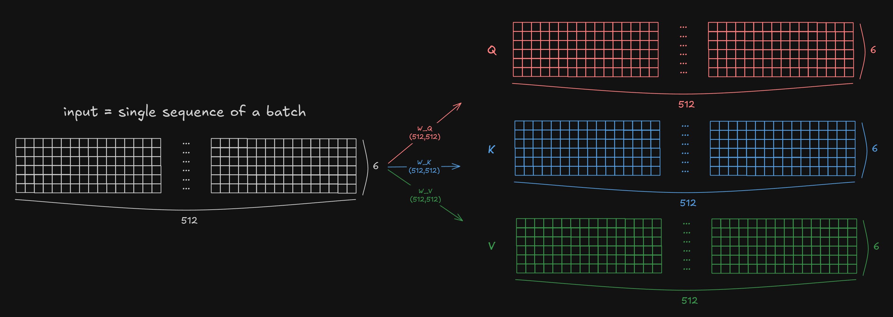
(d_model, d_k) each. However when implementing in code, it’s convenient to create a single combined weight matrix of size (d_model, d_model) for all heads, then split after projection. Also note that while Q,K,V are per-token (with sequence length seq_len), $W_Q, W_K, W_V$ are shared across all tokens within each head.2-1-2. Split heads
As mentioned above each h is d_model // d_k so we need to split d_model into h × d_k):
shape: (nbatches, n_seq_src, d_model) → (nbatches, n_seq_src, h, d_k)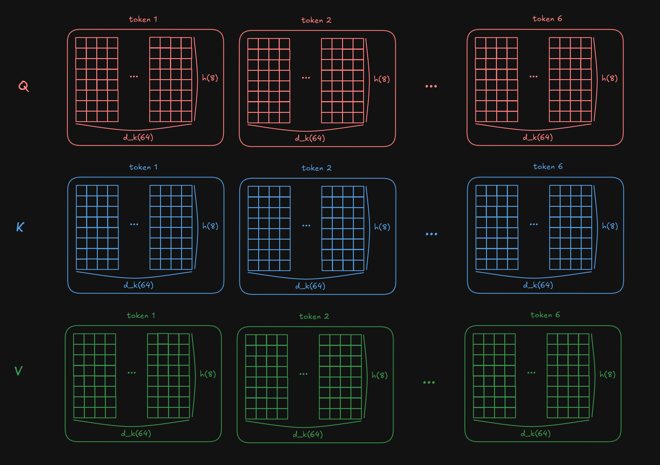
2-1-3. Transpose sequence length with head
We transpose the sequence length with head in order to parallelize head processing.
shape: (nbatches, n_seq_src, h, d_k) → (nbatches, h, n_seq_src, d_k)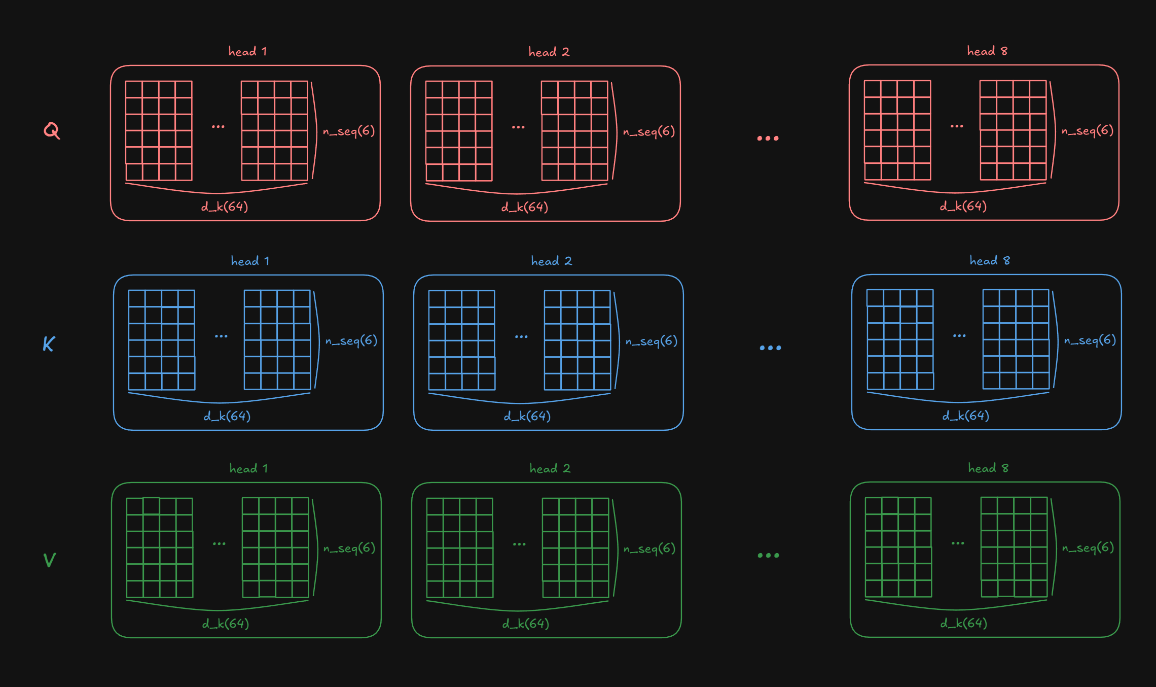
2-1-4. Compute attention scores
Attention score is calculated by $\text{softmax}(\frac{QK^T}{\sqrt{d_k}})$. Since $\sqrt{d_k}$ is just for scaling, if we look at $QK^T$, we are matrix multiplying $Q$ ((nbatches, h, n_seq_src, d_k)) with $K^T$((nbatches, h, d_k, n_seq_src)). Therefore attention score for a single sequence, for each head, for each batch is size of n_seq x n_seq.(nbatches, h, n_seq_src, d_k) → (nbatches, h, n_seq_src, n_seq_src)
for each head: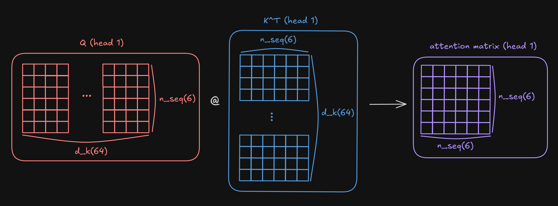
2-1-5. Softmax
Apply softmax function to the attention score (doesn’t affect the shape)(nbatches, h, n_seq_src, n_seq_src) (shapes unchanged)
2-1-6. Multiply by V
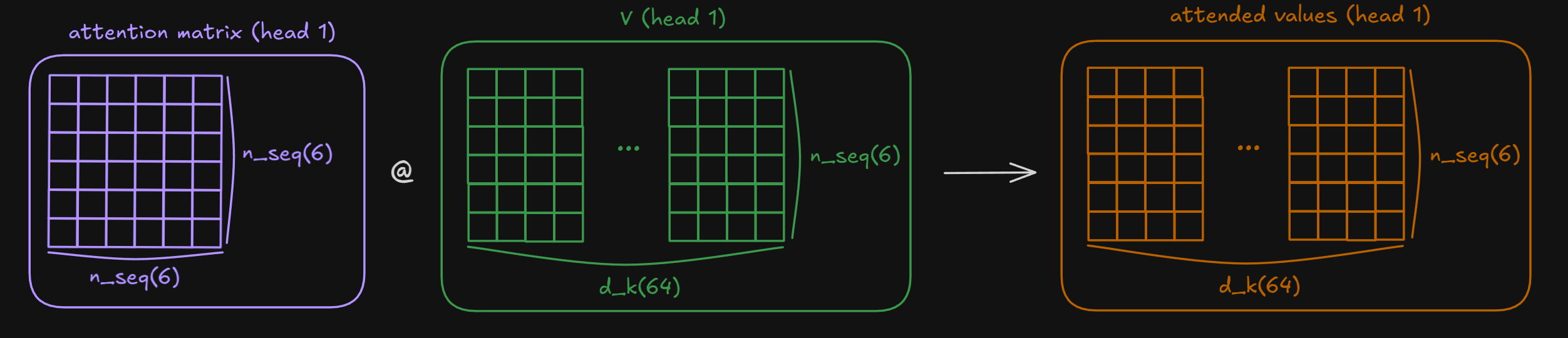
If attention score (calculated by $Q,K$) tells which token each token should “attend to”, $V$ tells which aspect/information to use from the token. We matrix multiply Attention Score with shape (nbatches, h, n_seq_src, n_seq_src) with V of shape (nbatches, h, n_seq_src, d_k) thus resulting as:(nbatches, h, n_seq_src, n_seq_src) → (nbatches, h, n_seq_src, d_k)
2-1-7. Transpose back & concat
Now we need to transpose the order of h and n_seq_src again. This is because calculation for Multi Head Self Attention is finished and we want to concatenate each head’s output.(nbatches, h, n_seq_src, d_k) → (nbatches, n_seq_src, h, d_k) (transpose)(nbatches, n_seq_src, h, d_k) → (nbatches, n_seq_src, d_model) (concat)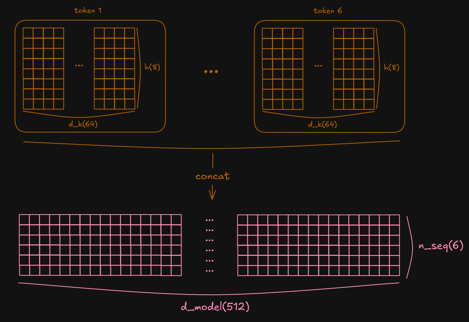
2-1-8. Forward Pass to O
After concatenating, we forward pass the batch into W_O.
W_O and why do we need it?A. After concatenation, each head’s output simply sits side-by-side without interaction.
W_O allows Cross-head integration – allows the model to learn combinations across different heads. e.g., combining a syntactic pattern captured by head 2 with a semantic pattern from head 5.W_O is shape of (d_model, d_model) so there is no shape change during this process.
shape: (nbatches, n_seq_src, d_model) (shapes unchanged)
If we look the code implementation of Annotated Transformer,
class MultiHeadedAttention(nn.Module):
    def __init__(self, h, d_model, dropout=0.1):
        "Take in model size and number of heads."
        super(MultiHeadedAttention, self).__init__()
        assert d_model % h == 0
        self.d_k = d_model // h
        self.h = h
        self.linears = clones(nn.Linear(d_model, d_model), 4)
        self.attn = None
        self.dropout = nn.Dropout(p=dropout)

    def forward(self, query, key, value, mask=None):
        "Implements Figure 2"
        if mask is not None:
            # Same mask applied to all h heads.
            mask = mask.unsqueeze(1)
        nbatches = query.size(0)

        # 1) Do all the linear projections in batch from d_model => h x d_k
        query, key, value = [
            lin(x).view(nbatches, -1, self.h, self.d_k).transpose(1, 2)
            for lin, x in zip(self.linears, (query, key, value))
        ]

        # 2) Apply attention on all the projected vectors in batch.
        x, self.attn = attention(
            query, key, value, mask=mask, dropout=self.dropout
        )

        # 3) "Concat" using a view and apply a final linear.
        x = (
            x.transpose(1, 2)
            .contiguous()
            .view(nbatches, -1, self.h * self.d_k)
        )
        del query
        del key
        del value
        return self.linears[-1](x)
If we look this code step by step,
        # 1) Do all the linear projections in batch from d_model => h x d_k
        query, key, value = [
            lin(x).view(nbatches, -1, self.h, self.d_k).transpose(1, 2)
            for lin, x in zip(self.linears, (query, key, value))
        ]
For convenience, we create four identical Linear layers of shape (d_model, d_model) to represent $W_Q, W_K, W_V$, and $W_O$ storing them in a ModuleList.
We then zip this list with the tuple (query, key, value). Since zip stops at the shortest iterator, it only iterates three times, effectively using the first three layers for $Q, K, V$ and leaving the fourth($W_O$) for later.
Inside the loop, we pass each input x through its corresponding linear layer lin. As defined in __init__, the output shape remains (nbatches, n_seq, d_model) (Step 2-1-1). Next we use .view() to split d_model dimension into h and d_k(Step 2-1-2). Finally we transpose the sequence length(n_seq) and head dimensions(h) using .transpose(1,2) to prepare for parallel head processing(2-1-3).
        # 2) Apply attention on all the projected vectors in batch.
        x, self.attn = attention(
            query, key, value, mask=mask, dropout=self.dropout
        )
Here, we call the attention function to calculate the attention scores and the final context vector (Step 2-1-4).
Let’s look at how this is implemented in the attention function:
def attention(query, key, value, mask=None, dropout=None):
    "Compute 'Scaled Dot Product Attention'"
    # ... (code omitted for brevity)
    scores = torch.matmul(query, key.transpose(-2, -1)) / math.sqrt(d_k)
    # ...
    p_attn = scores.softmax(dim=-1)
	# ...
    return torch.matmul(p_attn, value), p_attn
Both query and key enter with shape (nbatches, h, n_seq, d_k). We transpose the key tensor to (nbatches, h, d_k, n_seq). Performing matrix multiplication (matmul) between them results in the attention score matrix of shape (nbatches, h, n_seq, n_seq).
Next, we apply softmax to these scores (Step 2-1-5). We use dim=-1 to normalize the scores across the last dimension (the key positions), ensuring the attention weights for each query token sum to 1. Finally, we multiply these normalized weights by value to obtain the weighted sum (Step 2-1-6).
        # 3) "Concat" using a view and apply a final linear.
        x = (
            x.transpose(1, 2)
            .contiguous()
            .view(nbatches, -1, self.h * self.d_k)
        )
        del query
        del key
        del value
        return self.linears[-1](x)
Back in the MultiHeadedAttention code, we reverse the previous transpose operation and concatenate the heads to restore the shape (nbatches, n_seq, d_model) (Step 2-1-7). The .contiguous() call is necessary here to ensure the tensor’s memory layout is compatible with .view().
The del statements are included for memory efficiency, clearing references to large tensors to prevent memory spikes on the GPU11. Finally, we pass the concatenated result through the last linear layer in self.linears (which represents $W_O$) to mix the information from different heads (Step 2-1-8).
Residual + LayerNorm
After each submodules in Encoder finishes, we use residual connection and LayerNorm. There is no shape change in this process.
shape: (nbatches, n_seq_src, d_model) (shapes unchanged)
2-2. Feed Forward Network (FFN)
This works as a simple 2-Layer MLP which expands from d_model to d_ff and the final output returns to d_model.
2-2-1. Linear Layer(nbatches, n_seq_src, d_model) → (nbatches, n_seq_src, d_ff)
2-2-2. ReLU (or GELU)
Used as activation function between the two layers.(nbatches, n_seq_src, d_ff) (shapes unchanged)
2-2-3. Linear Layer(nbatches, n_seq_src, d_ff) → (nbatches, n_seq_src, d_model)
Residual + LayerNorm
Same as above(nbatches, n_seq_src, d_model) → (nbatches, n_seq_src, d_model)
3. Decoder Embedding Layer
Decoder Embedding Layer also embeds the tokens for the output. If we only consider the scope of “training”, we already have the targetting sequence. We want to embed them as well and use it to train the model to predict the next token. I will write this sequence as n_seq_tgt instead of n_seq_src to differentiate the two sources. Besides this name change, embedding layer works the same so I will skip duplicate explanation.
3-1. Token Embedding(nbatches, n_seq_tgt) → (nbatches, n_seq_tgt, d_model)
3-2. Positional Embedding(nbatches, n_seq_tgt, d_model) → (nbatches, n_seq_tgt, d_model)
4. Decoder Layer
Decoder Layer is consisted of three submodules which are:
4-1. Masked Multi-Head Self Attention
4-2. Cross Attention
4-3. Feed Forward Network.
Decoder Layer is repeated $N$(e.g., 6) times.
4-1. Masked Multi-Head Self Attention
Input from 3-2(nbatches, n_seq_tgt, d_model) (shapes unchanged)
Steps 1 ~ 4 works exactly the same as Encoder’s MHA (Forward $\rightarrow$ Split $\rightarrow$ Transpose $\rightarrow$ Score).
4-1-5. Masking
Mask is applied to the Attention Score matrix(of size n_seq_tgt, n_seq_tgt for each heads). Causal mask is an upper-triangular matrix of -inf values that prevents position i from attending to any position j > i. This prevents the model to “cheat” and ensures each token can only attend to itself and previous tokens.(nbatches, h, n_seq_tgt, n_seq_tgt) (shapes unchanged)
Steps 6 ~ 9 works exactly the same as Encoder’s MHA (Softmax $\rightarrow$ Multiply V $\rightarrow$ Concat $\rightarrow$ Forward O).
Residual + LayerNorm
4-2. Cross (Encoder–Decoder) Attention
What is Cross Attention?
Unlike Self-Attention where $Q, K, V$ all come from the same source, Cross Attention uses $Q$ from Decoder and $K, V$ from Encoder – the encoded source sequence.
This allows each decoder position to attend to all encoder positions, enabling the decoder to extract relevant information from the source sequence.
Input from 2(Encoder Layer) & 4-1(Masked Multi-Head Attention)
Input for $Q$: (nbatches, n_seq_tgt, d_model)
Input for $K,V$: (nbatches, n_seq_src, d_model)
4-2-1. Forward Pass to Q,K,V
$Q$: (nbatches, n_seq_tgt, d_model)
$K,V$: (nbatches, n_seq_src, d_model)
4-2-2. Split heads
$Q$: (nbatches, n_seq_tgt, d_model) → (nbatches, n_seq_tgt, h, d_k)
$K,V$: (nbatches, n_seq_src, d_model) → (nbatches, n_seq_src, h, d_k)
4-2-3. Transpose sequence length with head
$Q$: (nbatches, n_seq_tgt, h, d_k) → (nbatches, h, n_seq_tgt, d_k)
$K,V$: (nbatches, n_seq_src, h, d_k) → (nbatches, h, n_seq_src, d_k)
4-2-4. Compute attention scores
Since $QK^T$ is (nbatches, h, n_seq_tgt, d_k) $\cdot$ (nbatches, h, d_k, n_seq_src):(nbatches, h, n_seq_tgt, d_k) → (nbatches, h, n_seq_tgt, n_seq_src)
4-2-5. Softmax(nbatches, h, n_seq_tgt, n_seq_src) (shapes unchanged)
4-2-6. Multiply by V(nbatches, h, n_seq_tgt, n_seq_src) × V (nbatches, h, n_seq_src, d_k):(nbatches, h, n_seq_tgt, n_seq_src) → (nbatches, h, n_seq_tgt, d_k)
4-2-7. Transpose back & concat(nbatches, h, n_seq_tgt, d_k) → (nbatches, n_seq_tgt, h, d_k) (transpose)(nbatches, n_seq_tgt, h, d_k) → (nbatches, n_seq_tgt, d_model) (concat)
4-2-8. Forward Pass to O(nbatches, n_seq_tgt, d_model) (shapes unchanged)
Residual + LayerNorm: After each submodules in Encoder finishes, we use residual connection and LayerNorm. There is no shape change in this process.(nbatches, n_seq_tgt, d_model) (shapes unchanged)
4-3. Feed Forward Network (FFN)
Works exactly same as 2-2 (Feed Forward Network).
5. LM Head (Generator)
After $N$ (e.g., 6) steps of Decoder process is done, the decoder’s output is projected back into the vocabulary space in order to calculate the probability scores of the next token.
5-1. Linear Layer
We want to project the d_model for each token into token space vocab. So after passing this to the linear layer the shape changes:(nbatches, n_seq_tgt, d_model) → (nbatches, n_seq_tgt, vocab)
5-2. Softmax
We want the model to predict the next token in a stochastic way so we imply softmax function as well.(nbatches, n_seq_tgt, d_model) → (nbatches, n_seq_tgt, vocab)
Inference
During inference, we select the next token from this distribution using a decoding strategy (greedy, top-k, nucleus sampling, etc.) and feed it back as input to generate the next token autoregressively.
Training
During training, we don’t select tokens. Instead we directly compute cross-entropy loss between the predicted distribution and ground truth, then backpropagate to update weights.
Conclusion
We have gone through the common notations used in transformer, and used specific example to go through “one training phase” of Transformer Architecture. Finally we saw how shape changes in actual code (why all those reshape and transpose are used). Hope this post helps you gain insight and intuition of the bigger picture.